
There are two ways to create a quick filter for the bubble chart layer in the Excel Map: if you are Excel 2013+ user, you can create a slicer or you can create a non-standard filter based on your list.
Create a slicer on a Data table
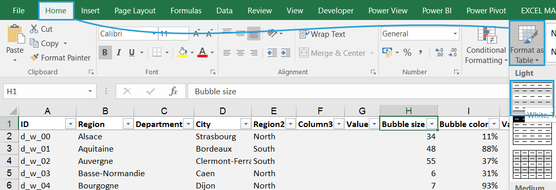
If you are an Excel 2013+ user then you are lucky – it’s really easy to create a slicer filter on a table. Because the bubble chart is connected with the Data sheet, you simply turn that sheet into a table and create a slicer.
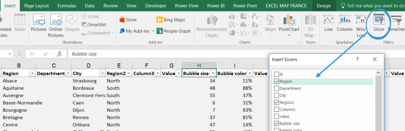
The slicer filters then the source table what makes the bubble chart show only the desired results.
By using a numeric slicer you can even limit the values on the bubble chart to values above or below the desired threshold – you just need to select all the values with Shift key on your keyboard:
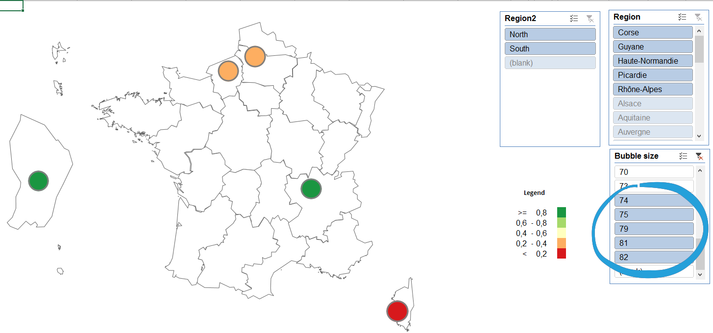
The problem with this filtering approach is that Excel is not showing the labels and on-click tooltip properly. That’s why you may need to check the second option for filtering the bubble chart – creating a formula filter.
Create a formula filter to get labels and tooltip
A formula filter approach means that you will have to create a combination of formulas to filter out the Data sheet. If you meet the conditions, the bubble gets the desired value, if not the bubble value needs to be 0. We will create a simple drop down to show values for the regions.
We start with adding the combo box (drop down) from Excel’s Developer tab (if you don’t see this tab, you can edit the ribbon and make it visible). After you right click it, you can go to Control tab and connect the drop down to the input and output cells.
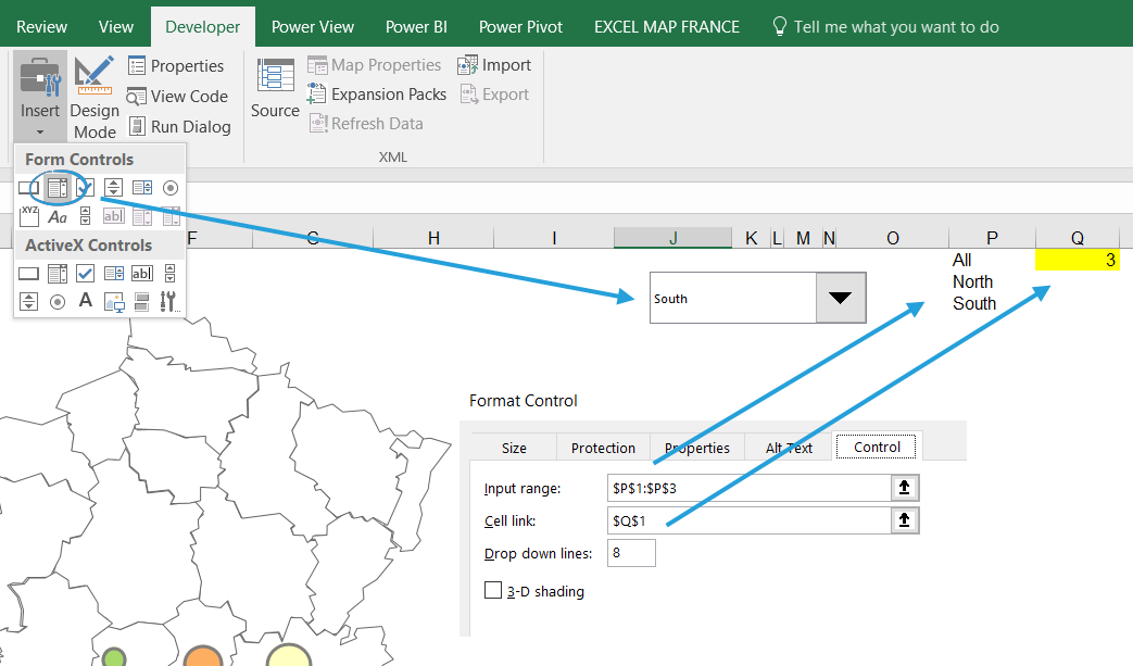
Then prepare a formula that based on your choices on a drop down will show either the bubble size or 0. In my example, where Q1 cell in the Map sheet is my output cell and E column of the Data sheet contains my Region names the formula will be as follows:
=IF(Map!$Q$1=1;Data!J2;IF(AND(Map!$Q$1=2;Data!E2=”North”);Data!J2;IF(AND(Map!$Q$1=3;Data!E2=”South”);Data!J2;0)))

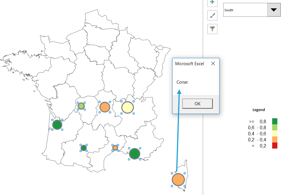
After copying the formula to the end of my data range I can test how my drop down works.
Watch the video tutorial to learn how to use the Excel Map
How to filter the bubble chart on Excel Map France?
Loading the video connects your browser to YouTube. YouTube may store data on your device.
Watch on YouTube instead