How to change the shape labels? – Example for Excel Map France

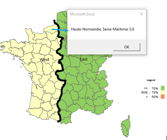
The default label in Excel Map, that is shown after clicking the shape (or a point on bubble chart), shows the name of the area, its parent (if there is any) and the value that can be found in the column G of Data sheet. How to edit this label?

The default shape label in Excel Map

The default label is shown below:

Edit the label

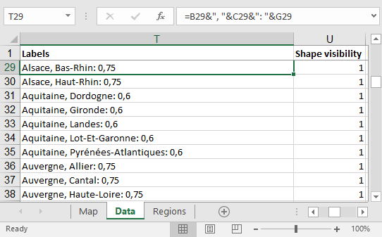
You can easily update it to show more information than this. To do so check the formula in column T of the Data sheet.

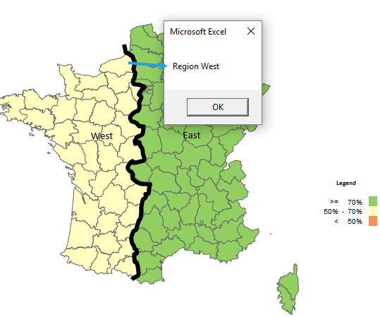
Let’s start with adding there information on region name (region has been created in column E of the Data sheet in the previous article on custom regions in Excel map) and results of the region. This example is based on Excel Map France so the cells addresses refer to Department level of France division.

=”Region “&E29

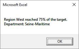
In the advanced example you can use a combination of many functions to get the desired result, like:

=”Region “&E29&” reached “&ROUND(G29*100;1)&”% of the target.”

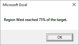
You can even enter new lines by using Excel CHAR function for a character number 10:

=”Region “&E29&” reached “&ROUND(G29*100;1)&”% of the target.”&CHAR(10)&”Department: “&C29

Watch the video tutorial to learn how to use the Excel Map

← All tutorials